Time Series Forecasting of Agricultural Product Prices Using Elman and Jordan Recurrent Neural Networks

This article is a summary of the scientific work published by Tetiana Kmytiuk, Ginta Majore

The original source can be accessed via DOI: 10.33111/nfmte.2021.067

Introduction

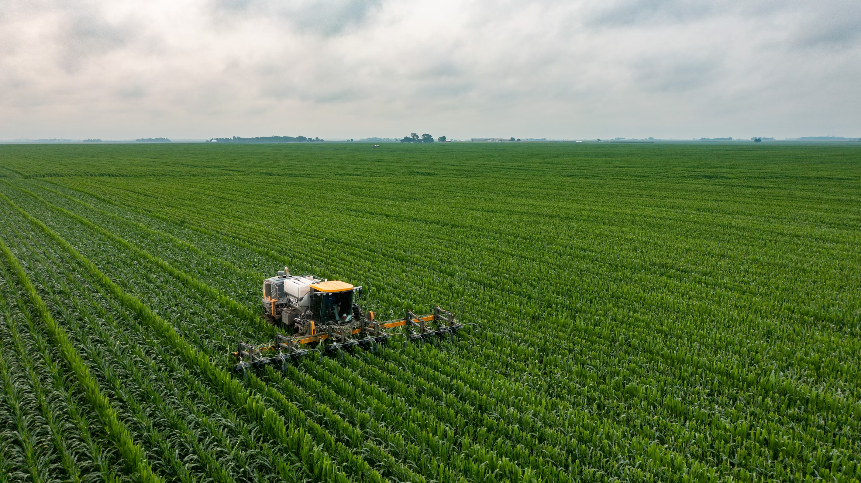
The agricultural market doesn’t sit still. Prices shift rapidly under the weight of unpredictable forces — weather, seasonality, shifting demand, supply chain disruptions, and even market sentiment. For producers, buyers, and policy makers, one thing is clear: accurate price forecasting isn’t just helpful — it’s critical.

But forecasting agricultural product prices is no easy task. Traditional economic models often fall short when faced with the nonlinear, volatile, and often chaotic nature of agri-market data. That’s why researchers have spent decades refining models that balance economic theory with statistical rigor — and, more recently, with artificial intelligence.

Over the years, forecasting techniques have ranged from classical time series models to fuzzy logic–based economic systems. But many of these tools come with baggage: complex math, sensitivity to parameter tuning, or a heavy reliance on domain-specific knowledge.

That’s where artificial neural networks (ANNs) step in — offering a flexible, self-learning alternative that can adapt to messy, real-world data. These models don’t need perfect assumptions or manually crafted rules. Instead, they learn patterns directly from the data itself — especially useful when relationships between variables are hidden, nonlinear, or just plain fuzzy.

In the world of time series forecasting, ANNs are usually deployed in two major forms:

• Feedforward networks, like multilayer perceptrons or convolutional neural nets, which process data in one direction.
• Recurrent neural networks (RNNs), which are uniquely equipped to handle sequences — and thus, ideal for predicting market behavior over time.

Unlike feedforward models, RNNs have memory. They can loop past information forward, allowing the model to "remember" what happened previously. This makes them especially effective for price forecasting, where historical trends and short-term fluctuations both matter.

In this study, we focus on two powerful types of RNNs: the Elman Neural Network (ENN) and the Jordan Neural Network (JNN). Both are designed to retain information over time, making them particularly well-suited for understanding the rhythm and volatility of crop markets.

We applied these models to a real-world case: predicting the future price of potatoes, one of the most economically significant agricultural products. Our goal? To test and compare the forecasting accuracy of ENN and JNN — and determine whether these tools can offer practical, reliable support for agricultural enterprises seeking to stabilize operations and make smarter pricing decisions.

Methodology: Recurrent Neural Networks for Time Series Forecasting

Recurrent neural networks (RNNs) represent a class of artificial intelligence models designed to process sequential data. Unlike traditional feed-forward networks, RNNs retain information from earlier steps, enabling the analysis of time series where past values influence future outcomes. This property makes them particularly suitable for forecasting in dynamic markets such as agriculture.

Several architectural forms of RNNs exist: one-to-one, one-to-many, many-to-one, and many-to-many. The defining characteristic of RNNs is feedback, which allows the network to capture dependencies across time. In contrast, feed-forward networks treat each input independently, without regard for earlier states. RNNs also apply shared parameters across time steps, improving efficiency and consistency when modeling sequences.

The design of an RNN involves the use of activation functions, which control how input signals are transformed into outputs. Common activation functions include the sigmoid function, the hyperbolic tangent, and the rectified linear unit (ReLU). The choice of activation function influences how effectively the model learns patterns in the data.

Two recurrent network types often applied in time series forecasting are the Elman and Jordan models. Both are designed to handle short-term memory in sequential data. The Elman model processes context information from the hidden layer, whereas the Jordan model uses information from the output layer. These differences allow the networks to capture varying aspects of time-dependent patterns.

Before use, RNNs must undergo training. This process consists of feeding historical data into the network, comparing predicted values with actual outcomes, and adjusting internal parameters to reduce error. Over repeated iterations, the network aligns its predictions more closely with observed values.

The training procedure follows several steps. First, input data are normalized to fall within a standard range, improving stability during training. Next, normalized values are introduced into the input layer. Finally, hidden layer states are computed based on both current inputs and previously processed information. Through this iterative process, the model learns to approximate the underlying structure of the time series.

Elman Neural Network (ENN)

The Elman neural network is a type of recurrent neural network architecture that extends the standard multilayer perceptron by incorporating a context layer. First introduced in 1990, this model includes one hidden layer and one context layer, which together enable the network to account for temporal dynamics in input data.

The network architecture comprises four layers: input, hidden, context, and output. The input layer consists of m neurons, while the hidden and context layers each contain n neurons. The output layer has a single neuron. The context layer mirrors the hidden layer’s structure and stores its previous state, allowing temporal information to influence future activations. This configuration provides the ability to track and use past states of the system when generating current outputs, improving prediction and control in dynamic processes.

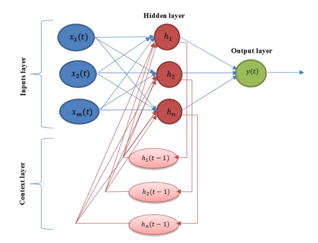
In this model, the input signal is processed step-by-step. Each signal activates the neurons of the hidden layer, the result is passed to the output layer, and the hidden layer’s state is copied to the context layer for use in the next step. This feedback loop forms the core of the network’s ability to capture time dependencies.

The mathematical model of the Elman network describes the hidden layer's activation as a function of both current input and past hidden states. The context layer provides delayed versions of the hidden outputs, which are combined with new inputs to update the hidden layer. The output is then calculated based on a weighted sum of the hidden neurons’ activations. The activation function, often a sigmoid, introduces non-linearity into the model. Weight parameters control the influence between layers and are optimized during training.

The Elman architecture supports tasks that require sequential data interpretation, including time-series forecasting, dynamic system modeling, and adaptive control. Its recurrent feedback mechanism enables more accurate modeling of systems where current outputs depend not only on present inputs but also on historical patterns.

Jordan Neural Networks (JNN)

Jordan neural network is a type of recurrent neural architecture derived from a multilayer perceptron. Unlike the Elman model, the Jordan network incorporates feedback from the output layer. Specifically, in addition to the input vector, a delayed version of the output is also fed back to the network’s input through a context layer. This delay can span one or several time steps.

The primary distinction lies in the memory mechanism: the Jordan model stores past outputs in the context layer, while the Elman model stores past hidden states. The architecture of the Jordan recurrent neural network is presented in Figure 3.

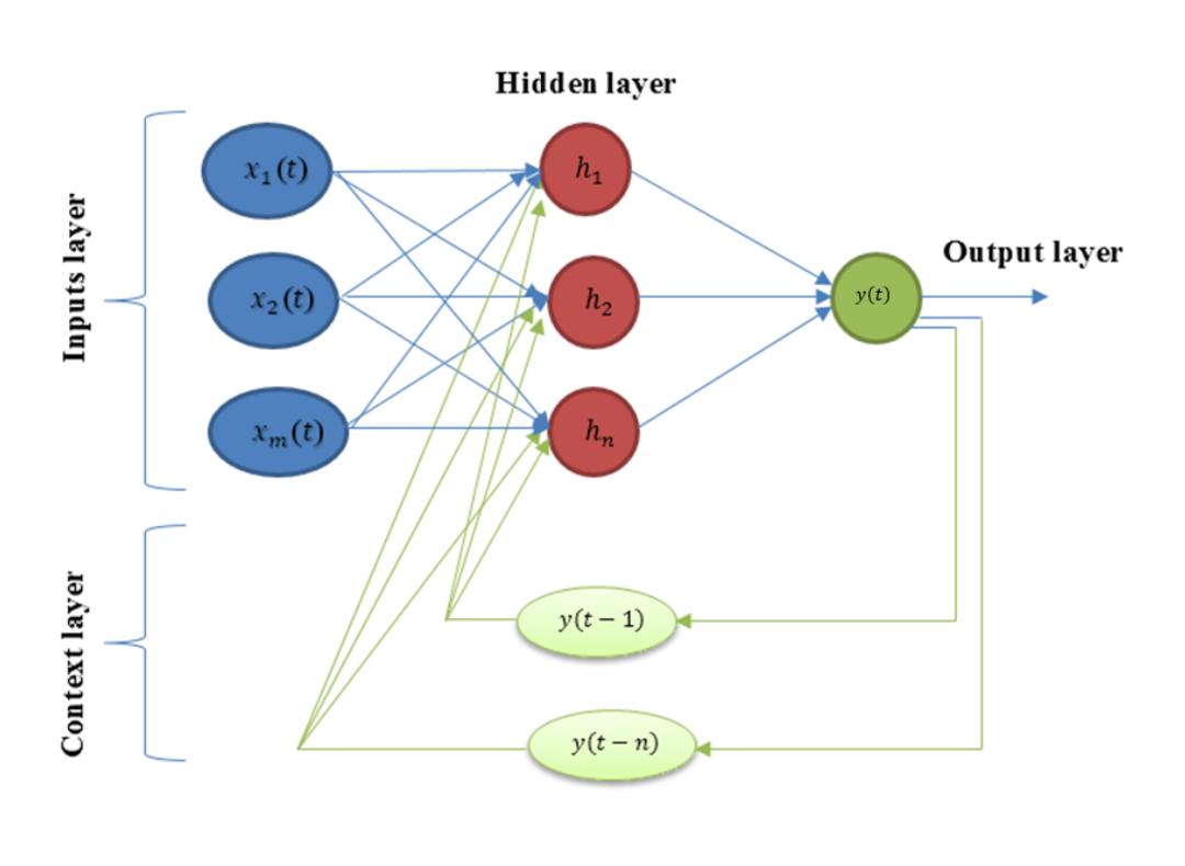
Signal processing within the Jordan model follows a specific sequence. The input layer receives the initial signal, which is then passed to the hidden layer. The hidden layer processes the input and transmits the result to the output layer. The output at time t is not only used as the final result but also stored and delayed in the context layer. During the next step, this delayed output is reintroduced as additional input to the hidden layer, along with the new input signal.

Mathematically, the Jordan model uses a similar formulation to the Elman model, with the key difference being the source of feedback. Instead of previous hidden states, the delayed output values are used in the recurrence. This leads to a dynamic system described by a set of nonlinear matrix equations. The equation for the hidden layer in the Jordan model includes terms from the input vector and delayed output values. The output layer is calculated based on the hidden layer activations.

One notable drawback of the Jordan network is its sensitivity to the depth of feedback. The number of context units required depends on how long the model must retain memory of the output sequence. This depth is not known in advance and can be difficult to optimize, presenting a challenge in practical applications.

Training the RNN

Training the Elman and Jordan recurrent neural networks for time series forecasting follows a structured multi-step process:

Step 1. Data collection and exploration.
This stage involves identifying the objective, collecting data, and analyzing their types and characteristics. Relationships between variables, dataset structure, outliers, and distribution patterns are examined. Decisions are made regarding the mathematical formulation of the forecasting model and the type of neural network architecture to apply.

Step 2. Model training.
Neural networks are trained through iterative optimization on a reference dataset to minimize prediction error. The dataset is typically split into training and testing subsets. The training subset is used to estimate model parameters, while the test subset is used to evaluate accuracy. The sampling process is random, ensuring a reliable performance assessment. At this stage, the number of hidden layer units and the presence of feedback mechanisms are selected.

Step 3. Model performance evaluation.
Evaluation techniques are applied to measure model accuracy and compare different forecasting architectures. Performance metrics and visualizations, such as error plots, highlight the gap between predicted and actual values. These insights guide the evaluation of each model’s forecasting capability.

Step 4. Conclusion and refinement.
Based on the evaluation results, conclusions are drawn and decisions are made on whether to refine the model or proceed to its practical implementation.

Model prediction accuracy

Forecast accuracy is typically evaluated using statistical error metrics. In this study, the performance of Elman and Jordan neural networks is assessed by computing three key evaluation criteria: mean square error (MSE), root mean squared error (RMSE), and mean absolute error (MAE).

These indicators reflect the deviation between predicted and actual values, offering a quantifiable way to compare model precision. Table 1 presents the definitions and formulas used for each criterion.

Smaller values of these indicators correspond to higher forecasting accuracy.

Results and Discussion

The prediction process started with preparing the dataset. We used data on the average monthly retail prices of potatoes in Latvia, covering the period from January 2005 to July 2021. The dataset included 199 data records in total.

All analyses were conducted using the R programming language. The time series data was decomposed into separate components using the stl function from the stats package. The forecasting models were built using two types of recurrent neural networks — Elman and Jordan — via the RSNNS package.

Fig. 4 shows the original time series plot. A clear upward trend is visible, along with strong seasonality in the data.

To better understand the underlying structure, we decomposed the time series into its three main components: trend, seasonality, and residual noise. These are shown in Fig. 5.

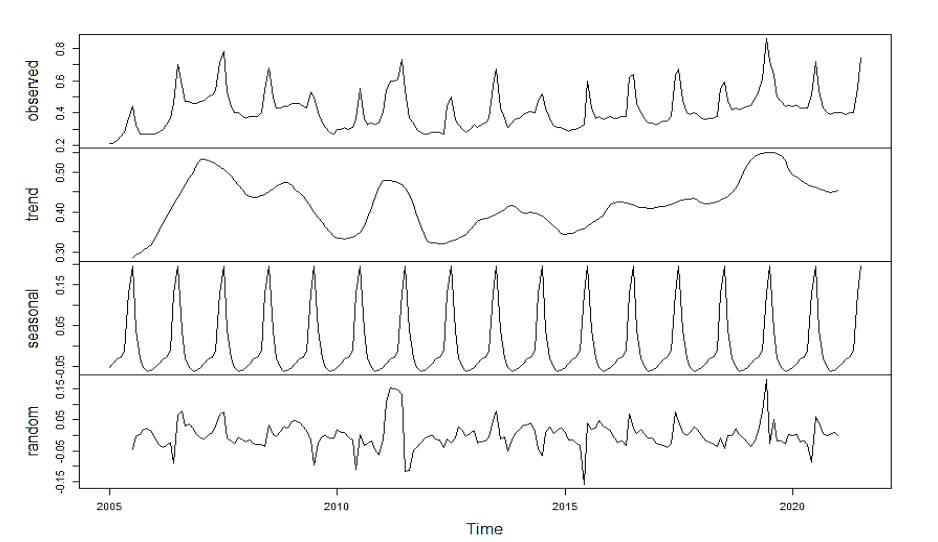
As shown in the decomposition, seasonal fluctuations repeat every 12 months. Price spikes are typically observed during the summer months. Based on the monthly frequency of the data, we created 12 time-lag variables to serve as input features for the neural networks.

The dataset was split into training and testing sets. We followed a standard approach: 70% of the data was used for training, and the remaining 30% for testing. The architecture of both Elman and Jordan networks included three layers: input, hidden, and output. We tested different network configurations and chose the optimal structure through trial and error. The final architecture included 12 input neurons (representing the 12 previous months), 2 hidden neurons, and 1 output neuron predicting the next value.

Table 2 summarizes the key parameters of the training dataset and neural networks.

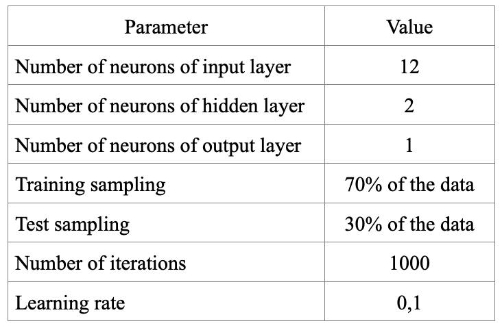
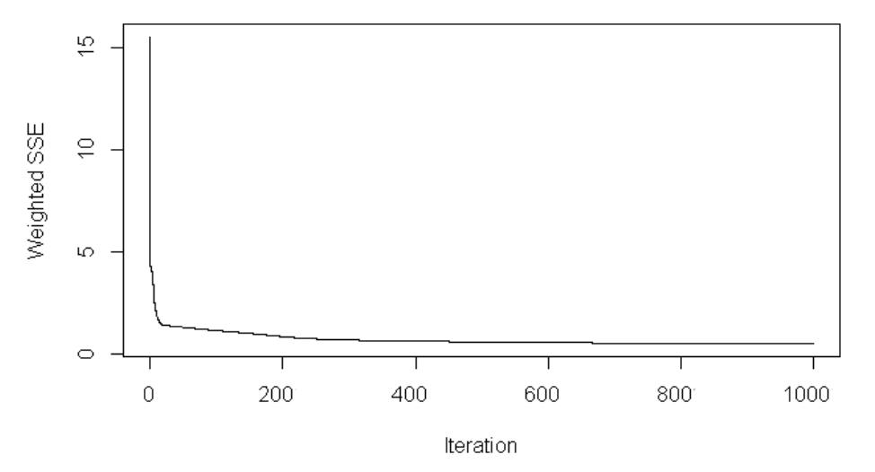
Both models were trained for 1000 iterations, using a learning rate of 0.1. Fig. 6 and Fig. 7 show the error curves during training for the Elman and Jordan networks, respectively. Both models show a clear decrease in error during training. The Elman model stabilizes early and reaches a low error level, while the Jordan model shows a more gradual decline.

We further evaluated both models using regression error plots. Fig. 8 displays the relationship between the predicted and actual values for the Elman network. The predicted values align closely with the actual ones, which indicates a strong fit to the training data. The correlation coefficient squared (R²) was 0.83, confirming a strong relationship.

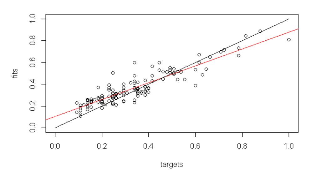
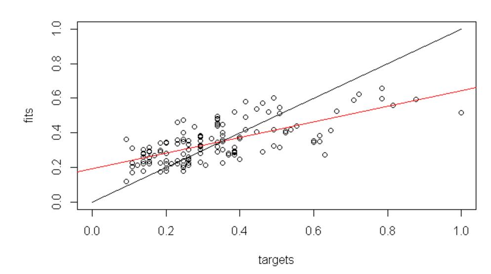
Fig. 9 shows the same regression plot for the Jordan network. The fit is visibly weaker, and the R² value drops to 0.59. While this is still a moderate level of correlation, it indicates the model does not fit the training data as well as the Elman network.

Next, we tested both models on unseen data to evaluate their forecasting performance. Fig. 10 shows the predicted versus actual values from the test set. The black line represents the true values, while the green and red lines represent the predictions made by the Elman and Jordan models, respectively.

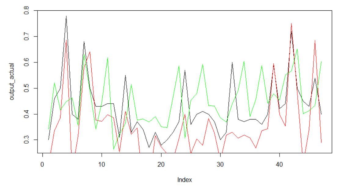
The Elman network shows better alignment with the actual values compared to the Jordan network. This is further confirmed by the correlation coefficient for the test set, which is approximately 0.78 for Elman. We also calculated MAE, MSE, and RMSE for both models. The results are presented in Tables 5 and 6.

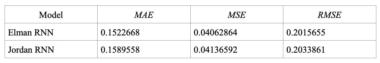
As shown in the tables, the Elman network consistently performs better than the Jordan network, both on training and test data. Its error values are lower across all three metrics. Based on this, we conclude that the Elman recurrent neural network is more accurate and effective for forecasting this type of agricultural time series.

Conclusion

This article addressed the task of predicting historical prices for agricultural products, using potatoes as a case study. The goal was to assess the applicability of Elman and Jordan recurrent neural networks for modeling such time series.

The findings show that both neural network architectures can effectively model time series data, even when trained on a randomly selected subset. Both the Elman and Jordan models demonstrated strong forecasting performance, as measured by standard statistical criteria such as MAE, MSE, and RMSE, across both the training and test datasets.

However, the Elman network consistently outperformed the Jordan network, delivering more accurate predictions of price dynamics. These results highlight the importance of selecting an appropriate neural architecture based on the specific problem and dataset.

In practice, designing an effective neural network model requires careful consideration of multiple factors, including the number of input variables, the structure of hidden and context layers, and the choice of activation functions.

Future research should focus on experimenting with alternative network configurations, expanding the dataset, and exploring hybrid models that combine Elman and Jordan architectures.