

AI Product Modernization Playbook · 07 / 12
A forecast becomes a product feature when it helps someone decide how much to order, which capacity to reserve or when to act. The prediction is one component of that decision, alongside uncertainty, operating constraints and the cost of being wrong.
Imagine a replenishment planner opening your product on Monday morning. A chart predicts next week's demand, but the supplier needs ten days to deliver, the warehouse already has stock in transit, and the next promotion has just changed. The chart may be statistically impressive and still leave the planner doing the real work in a spreadsheet.
This chapter of the AI Product Playbook explains how to build forecasting into an existing product: define the decision, reconstruct what was knowable at each point in time, evaluate realistic horizons, and connect predictions to a controlled planning workflow. Demand planning is the running example; the same principles apply to staffing, infrastructure capacity, sales and cash-flow planning.
On this page
1. Define the decision before the model
Start with a short decision contract that product, operations and engineering can all inspect. Specify the owner, the quantity being predicted, the unit of work, when the decision is made and what can still change afterward. “Predict sales” leaves almost every important question unanswered.
Make the time contract explicit
For replenishment, define whether the target is units sold or unconstrained demand, at which product–location level, and over which dates. The required horizon depends on supplier lead time and review frequency. A daily forecast for tomorrow cannot support an order whose stock arrives next week. Record the data cutoff, issue time, decision deadline, time zone and calendar rules, including holidays and daylight-saving transitions where relevant.
An illustrative contract might be: every Monday, recommend purchase quantities for a selected product category using information available by Sunday evening, while planners approve exceptions before the supplier deadline. The exact schedule and thresholds must come from the operation; this example is not a performance claim.
Choose an outcome the user can change
Pair a business objective with guardrails. Replenishment might reduce inventory while protecting availability. Staffing might reduce overtime while maintaining service levels. Capacity planning might reduce idle resources without increasing missed requests. Name who may accept, override or execute a recommendation. A forecast alone should not silently acquire permission to place orders.
2. Build an honest history of the target
The hardest forecasting errors often begin before model training. Product identifiers change, stores close temporarily, refunds arrive late, and “zero” can mean no demand, no inventory or no data. Define these states explicitly instead of filling every missing cell with zero.
Sales are not always demand
If an item sells out at noon, the observed sales total hides some of the demand that would have arrived later. Training directly on that total can teach the system to keep under-ordering. Preserve availability, stockout intervals, cancellations, backorders and substitution signals where available. Decide whether the product is forecasting realized sales under a given availability plan or estimating latent demand.
Any reconstruction of lost demand is an estimate. Keep it separate from observed sales, identify how it was produced, and test how planning decisions change under alternative assumptions. Simply discarding every stockout period can also bias evaluation toward easy, well-stocked periods. A pilot changes availability, so its observed sales may no longer be comparable with history under the previous ordering policy.
Maintain a consistent series registry with launch and retirement dates, category mappings, units and location changes. History should cover the patterns relevant to the decision, but there is no universal minimum number of years. A product with one seasonal cycle needs a different validation strategy from a mature portfolio with several cycles and many comparable items.
3. Reconstruct what was knowable at the cutoff
Every input needs both a business timestamp and an availability timestamp. A transaction that occurred on Friday but reached the platform on Tuesday was not available for Monday's forecast. Historical values can be legitimately corrected later; preserve the earlier versions so evaluation can replay the original information state.
Separate known future inputs from future observations
Calendar dates are known in advance. Promotions, prices and staffing plans are known only to the extent that their recorded versions existed at the forecast cutoff. Weather observations for next week are unavailable today; a weather-sensitive model needs the archived weather forecast issued at that time, or an explicit assumption about missing forecast vintages.
Build lagged and rolling features using only available history. Fit imputers, scaling rules, feature selection and tuning inside the appropriate training periods. Otherwise, leakage can enter through preprocessing even when the final train/test split looks chronological.
When historical input vintages are missing, document the limitation and run a prospective shadow period. A backtest built with today's corrected plans can still answer a restricted research question, but it cannot establish how the live system would have performed with the information actually available then.
4. Separate predictions from planning decisions
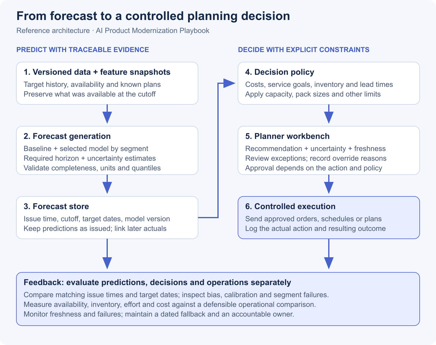
A useful architecture has a data layer, a forecasting service, a forecast store and a decision layer. Batch generation often fits scheduled planning well; interactive scenarios can run separately. The planner should see when a forecast was issued and whether its inputs are fresh, rather than waiting for an expensive model run every time a screen opens.
Keep a record of each forecast as issued
Store the series identifier, target definition, issue time, input cutoff, target dates, model and feature versions, training snapshot, baseline, and supported quantiles or distribution samples. A forecast for Friday issued on Monday is a different record from one issued on Thursday. Do not replace the earlier record with the newer prediction.
Keep actuals, policy recommendations and planner overrides as linked records. This makes it possible to distinguish a poor prediction from a sensible prediction used with the wrong lead time, a stale inventory balance or a manual intervention. Validate completeness, units, nonnegative quantities where required, and quantile ordering before exposing a run to the product.
5. Make advanced models earn their place
Establish a seasonal naive baseline and, where appropriate, simple statistical models such as exponential smoothing. Include the current planning process as an operational comparator. These are useful production fallbacks as well as evaluation references.
Select by segment and operating cost
Benchmark global boosted-tree models that learn across related series, specialist methods for intermittent demand, and neural or pretrained time-series models when their capabilities fit the problem. Compare accuracy, calibration, inference cost, refresh time and maintenance burden on the same historical cutoffs. A higher leaderboard score does not automatically justify a slower planning cycle.
Use a small, understandable routing policy if different segments need different models. A mature high-volume item, a sparse spare part and a new product need not share the same treatment. Evaluate cold starts by withholding entire product launches or entities in a way that mirrors onboarding; ordinary time splits on established series do not test that problem.
The M5 retail forecasting competition provides a useful historical example. Januschowski and colleagues report that winners in both tracks relied heavily on gradient-boosted trees. That supports including strong tabular baselines; it does not establish that trees win in every domain or against every newer model. See Forecasting with trees.
6. Backtest the decision horizon, not a convenient split
Use rolling forecast origins: train using information available at one historical cutoff, issue the required horizon, then move the cutoff forward and repeat. Hyndman and Athanasopoulos describe this approach in their forecasting toolbox. The practical requirement is to reproduce when your user could actually act.
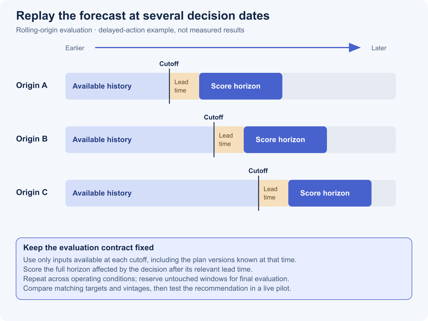
If decisions must be committed in advance, evaluate the dates they can affect. Keep relevant delivery or processing delays in the simulation. Replenishment also requires demand during lead time to project the stock available on arrival; evaluate cumulative demand over the full protection period instead of dropping that interval. Include ordinary periods, promotions, holidays and disruptions that matter to the business, while reporting when there are too few examples to draw a strong conclusion.
Protect the final evaluation
Use earlier windows for model and feature selection, then reserve later untouched windows for the final comparison. Repeatedly choosing the best model on the same “test” period turns that period into a tuning set. Overlapping forecast horizons also create dependent errors; do not present thousands of overlapping rows as thousands of independent experiments.
Replay the policy as well as the prediction where possible: stock on hand, incoming orders, ordering constraints and costs. Such simulations remain conditional on assumptions about lost demand, supply reliability and user behavior. Use them to select candidates and expose failure modes, then validate operational value prospectively.
7. Treat uncertainty as a product requirement
A single number hides the tradeoff between excess capacity and shortages. Offer a distribution or a small set of quantiles that the decision layer can use. Explain what each displayed statistic means: the median is not the mean, and a high quantile is not a promise that demand will stay below it.
Check coverage and usefulness together
A P10–P90 band has nominal central coverage of 80%. Measure realized coverage by horizon and meaningful segment, alongside interval width and quantile loss. Very wide intervals may cover most outcomes while providing little planning value. Sparse discrete counts and small samples also make exact nominal coverage difficult to interpret; show sample sizes and avoid false precision.
Calibration is an ongoing task when the operating environment changes. Gibbs and Candès' Adaptive Conformal Inference Under Distribution Shift studies adaptation of prediction sets and long-run coverage frequency. That result should not be presented as a guarantee of precise coverage for every product, subgroup or individual forecast. Monitor local failures and the width of the intervals users receive.
Define how uncertainty affects the interface: low-evidence forecasts may require review, while unsupported scenarios should say that the system lacks evidence. An empty band, a failed model run and a genuinely narrow interval are different product states.
8. Make totals and time horizons consistent
Planning often crosses product, category, store, region and company views. Establish which hierarchy applies at each historical date, and reconcile forecasts so compatible point predictions add up where the product requires coherence. The methods and tradeoffs are covered in Forecasting hierarchical and grouped time series.
Probabilities require extra care. Adding store-level P90 values does not generally produce the region's P90. Likewise, adding daily upper quantiles does not produce the upper quantile of cumulative lead-time demand. The distribution of a sum depends on how outcomes move together across locations and dates.
If the ordering policy needs total demand over a replenishment window, evaluate a direct cumulative forecast or appropriately dependent sample paths and probabilistic reconciliation. Test the aggregate distribution actually consumed by the policy. Coherent means or totals alone do not establish coherent uncertainty.
9. Translate forecasts into feasible recommendations
The decision layer combines the forecast with inventory position, expected deliveries, lead times, service objectives, storage limits, supplier minimums, pack sizes and the consequences of shortages or surplus. Version those assumptions alongside the recommendation so users can reconstruct why it changed.
Show the reasoning behind the quantity
In a deliberately simplified illustration, suppose the chosen quantile of demand over the protection period is 150 units and inventory position is 90. A provisional replenishment amount is 60 units before pack sizes, minimum orders, capacity and other constraints are applied. These numbers are illustrative, not observed results. The selected quantile must reflect the relevant costs or service policy and be validated; it should not be an arbitrary “conservative” setting.
Keep assumptions visible for what-if scenarios. A forecast conditional on a planned price or promotion does not automatically estimate the causal effect of changing that price or promotion. Historical associations and feature-importance explanations are insufficient to establish elasticity. Decisions that depend on causal effects need suitable experiments or a defensible causal model, with limits disclosed.
For irreversible commitments, show the proposed action, applicable constraints and required approval. Routine low-risk recommendations can become more automated after evidence supports that authority level. The authorization boundary belongs to the business workflow, independently of the model's confidence score.
10. Build a planner workbench, not just a chart
Give users an exception queue ordered by decision importance: likely shortages, unusually large changes, stale inputs, unsupported launches and unresolved constraints. Show the forecast range, baseline, relevant history, input freshness and the recommended action together. Separate a genuine demand shift from a change caused by a new model or revised plan.
Make overrides explicit and measurable
Record the affected dates, original forecast, changed value, owner, reason and expiry of every override. Distinguish a one-time event from a lasting assumption. Avoid silently folding all overrides into training labels; planners may know something the model does not, but they may also be expressing a target or commercial commitment rather than expected demand.
Assess forecast value added by comparing the baseline, model and final forecast on the same cases, issue times and target dates. Overrides tend to occur on difficult cases, so comparing the average error of overridden items with untouched items is misleading. Forecast value added measures forecast-process improvement; business value requires separate evidence about decisions and outcomes.
A conversational layer can retrieve forecasts, explain recorded drivers and help navigate scenarios. Have it call the forecasting service for numbers and preserve units, dates and versions in its answer. Generated narrative is not a substitute for a tested numerical pipeline. The workflow patterns in the copilot chapter apply directly to this interface.
11. Measure prediction quality and decision value
Use a scorecard that connects model behavior to the planner's job. Report performance by forecast horizon and segment, as well as the overall result. A high-volume category can hide severe failures in smaller but operationally critical segments.
Swipe horizontally to read all columns.
| Layer | What to measure | What to check before trusting it |
|---|---|---|
| Point forecasts | Absolute or scaled error, signed bias, improvement over baseline | Use matching cutoffs and horizons; inspect high- and low-volume segments. |
| Uncertainty | Quantile loss, interval coverage and width | Check horizon, segment, sample size and the aggregate distribution used by decisions. |
| Planning outcomes | Availability, stock, waste, overtime, missed demand or other decision-specific costs | Account for policy changes, constraints, censoring and differences between pilot groups. |
| User workflow | Review effort, exception resolution, overrides and decision turnaround | Measure whether users can act before the deadline and understand limitations. |
| Operations | Freshness, run completeness, latency, failures and cost | Verify the fallback works for the actual dates and decision being served. |
Metric denominators matter. MAPE breaks down around zero actuals; WAPE is undefined when total actual demand is zero and emphasizes large volumes. MASE and RMSSE need an explicit policy when their historical scaling denominator is zero. Document exclusions and report coverage of the scored population rather than quietly removing troublesome series.
A useful deployment example comes from DeepMind's 2019 wind-energy project. The team forecast output 36 hours ahead and used predictions to recommend hourly grid commitments a day in advance. It reported roughly 20% higher wind-energy value relative to a baseline without time-based commitments. This was a value comparison in that deployment, not a 20% increase in generated electricity or a universal accuracy claim. The transferable lesson is the connection between prediction and a specific decision. See DeepMind's original account.
12. Roll out with operating controls
Move from historical evaluation to shadow forecasts, then a limited assisted pilot. Before launch, agree on the comparison method, success criteria, guardrails and duration needed to observe outcomes. Randomization or matched comparisons may need to operate at store, team or region level when inventory, people or decisions are shared; otherwise treatment can spill into the control group.
Set criteria using local baselines rather than borrowed percentages. A pilot might require improved availability without exceeding an inventory limit, stable forecast delivery before the planning deadline, and an acceptable review workload. These are categories of acceptance criteria, not promised results or universal thresholds.
Design for stale data and failed runs
Monitor data arrival, schema changes, missing series, distribution shifts, bias and calibration as actuals mature. Assign an owner for both the model and the operating decision. Alerts need a response: investigate an upstream feed, switch to a validated baseline, route exceptions to planners or pause automated recommendations.
A last-known forecast is usable only if it still covers the target dates, meets an agreed age limit and remains appropriate for the current conditions. Never slide yesterday's values forward just to populate today's screen. Mark fallback mode clearly and log which decisions used it. For downstream execution, apply the bounded authority and recovery controls described in the agentic automation chapter.
13. Start with one decision and a complete feedback loop
A strong first release supports one recurring decision from end to end: an explicit target and horizon, trustworthy data snapshots, a baseline, a realistic backtest, useful uncertainty, a constrained recommendation and an interface that records what the planner actually did.
The minimum delivery package should include the decision contract, source and feature definitions, forecast-version schema, evaluation report, exception workflow and fallback runbook. Expand to additional segments or higher automation only when the evidence supports it. This creates a product capability that can be operated and improved, rather than a prediction demo that stops at a chart.
If you are adding forecasting to an existing product, start the implementation discussion with the decision users already make, the information they have at that moment and the consequences of a mistake. Those details determine the architecture more reliably than selecting a model first.
Next in the series: anomaly detection and monitoring—how to identify unusual behavior, prioritize useful alerts and connect detection to an effective response.
Sources and further reading
This article develops the forecasting chapter of the AI Product Playbook. Architectural patterns and numerical examples are implementation guidance, not claims about measured Infinity Technologies client outcomes. External examples and methodological references were checked against the following primary sources.
- Hyndman and Athanasopoulos, Forecasting: Principles and Practice — The forecaster's toolbox, for rolling-origin evaluation, forecast distributions and scoring.
- Hyndman and Athanasopoulos, Forecasting hierarchical and grouped time series, for aggregation and reconciliation.
- Januschowski and colleagues, Forecasting with trees, for the historical M5 competition findings.
- Gibbs and Candès, Adaptive Conformal Inference Under Distribution Shift, for online calibration and the scope of long-run coverage results.
- Elkin and Witherspoon, Google DeepMind, Machine learning can boost the value of wind energy, February 2019, for the forecast-to-commitment deployment example.