

AI Product Playbook · 11 of 12
A forecast tells a planner what might happen. An optimization feature helps them decide what to do: which orders to promise, how much capacity to reserve, where to allocate inventory, or which schedule to release.
Consider a distribution manager facing a demand spike. A dashboard can show tomorrow’s expected orders. A useful planning product goes further: it compares feasible delivery plans, exposes the cost of keeping reserve capacity, explains which commitments create bottlenecks, and lets the manager approve a plan that the operating system can actually execute.
Chapter 11 of the AI Product Modernization Playbook explores this move from prediction to decision. The implementation combines operations research, simulation, product design and, where useful, machine learning. Its central challenge is making the assumptions, constraints and consequences of a recommendation visible before the business commits to it.
On this page
1. Start with a decision contract
Choose one recurring decision with a clear owner, meaningful alternatives and a measurable outcome. “Optimize operations” is too broad. “Propose tomorrow’s delivery assignments for one depot, before the dispatch deadline, while meeting capacity and customer commitments” is a workable starting point.
Write down the planning horizon, decision frequency, deadline, editable variables, mandatory constraints, approval authority and destination system. Include the current manual or rule-based baseline. A faster recommendation has little value if the planner cannot inspect it before the dispatch window closes.
Separate four capabilities
- Forecasting estimates uncertain inputs, such as demand or travel time.
- Scenario analysis changes explicit assumptions and compares consequences: a supplier is late, capacity falls, or a promotion increases demand.
- Simulation evaluates how a proposed policy or plan might behave over time under modeled conditions.
- Optimization searches for a preferred decision under a specified objective and set of constraints.
These capabilities can work together, but they are not interchangeable. A simulation does not automatically find the best plan. An optimizer does not prove that its demand assumptions are correct. A useful first version may use a conventional solver and a simple baseline forecast without an LLM. The forecasting article in this series covers the upstream prediction problem.
2. Make objectives and constraints explicit
The objective is a product policy. Minimizing transport cost, maximizing completed orders and minimizing lateness can produce different assignments from identical data. Ask the decision owner to resolve these tradeoffs before encoding them.
Hard rules and priced preferences
Hard constraints define what the model permits: vehicle capacity, inventory availability, required qualifications or an approved operating limit. Soft constraints express preferences whose violations incur a documented penalty, such as a less convenient delivery slot. A rule does not become optional simply because satisfying it is expensive.
Give each rule a name, business owner, unit, source and effective date. Operations and the responsible specialists must validate the rule inventory, including applicable contractual and regulatory requirements. Mathematical feasibility only establishes consistency with the rules that were actually encoded.
For competing goals, use business-approved priorities or show several tradeoff options. If combining costs into one score, convert them into coherent units and expose the weights. An arbitrary weight can quietly make a missed delivery cheaper than hiring an available vehicle. For strict priorities, a hierarchical objective may express the policy more faithfully than one weighted sum.
Also account for plan stability. Moving a delivery to another driver may save distance while creating customer notifications, loading changes and confusion. Treat these consequences as explicit costs or change limits, rather than assuming every mathematically improved schedule should replace the last one.
3. Build a reproducible planning snapshot
A plan needs more than a forecast table. Assemble orders, inventory, locations, calendars, equipment availability, capacity, costs and eligibility rules into an immutable input snapshot. Record the time at which each input was known and the version of every forecast and policy.
Keep uncertainty attached to its inputs
Preserve forecast ranges or scenario samples when the decision depends on variability. A single expected demand value hides the difference between steady demand and a volatile distribution with the same mean. Preserve relevant relationships too: a storm can increase travel times across several routes at once.
Check identifiers, missing values, time zones, units and conflicting reservations before optimization. An unavailable truck mistakenly marked as available is a data defect, even if the resulting model solves perfectly. Define freshness limits and what happens when an essential feed is late.
Some scenarios change the system itself. Raising a price may change demand; changing a delivery promise may change order conversion. A correlation learned from past observations is not automatically an estimate of that intervention’s effect. Where causal response is uncertain, state the assumption and test a range rather than presenting one precise commercial outcome as established.
Store scenario changes as a readable difference from the baseline snapshot. “Two vehicles unavailable and demand 15% higher” is reviewable. An unexplained replacement input file is much harder to audit.
4. Match the method to the decision
Start with the structure of the problem and the time available to decide. The following is a selection guide, not a guarantee that one method will perform best on a particular workload.
| Decision structure | Candidate approach | Main implementation question |
|---|---|---|
| Divisible allocation with linear costs and limits | Linear programming | Are continuous quantities operationally meaningful? |
| Assignments, open/close choices or discrete quantities | Mixed-integer optimization | Can representative instances reach useful quality before the deadline? |
| Schedules with logical rules and sequencing | Constraint programming or CP-SAT | Are calendars, dependencies and integer units modeled correctly? |
| Large routing or scheduling searches | Specialized search and heuristics | How do feasible results compare with the baseline under the same time budget? |
| Uncertain demand, failures or travel times | Stochastic or robust formulations, plus simulation | Which scenarios or uncertainty sets are supported by evidence? |
Swipe horizontally to read the complete table.
Benchmark a straightforward formulation before adding sophistication. Some products need a good feasible plan in seconds; others can spend an hour evaluating a strategic allocation. Measure memory, latency and solution quality on small, typical and difficult instances. A solver demonstration on clean sample data does not establish production capacity.
Use a deterministic rule-based planner as a comparison and, where appropriate, a fallback. Its simplicity can make data and modeling errors easier to expose. Machine learning is most useful when it improves inputs or response models that materially affect the decision.
5. Separate planning from execution
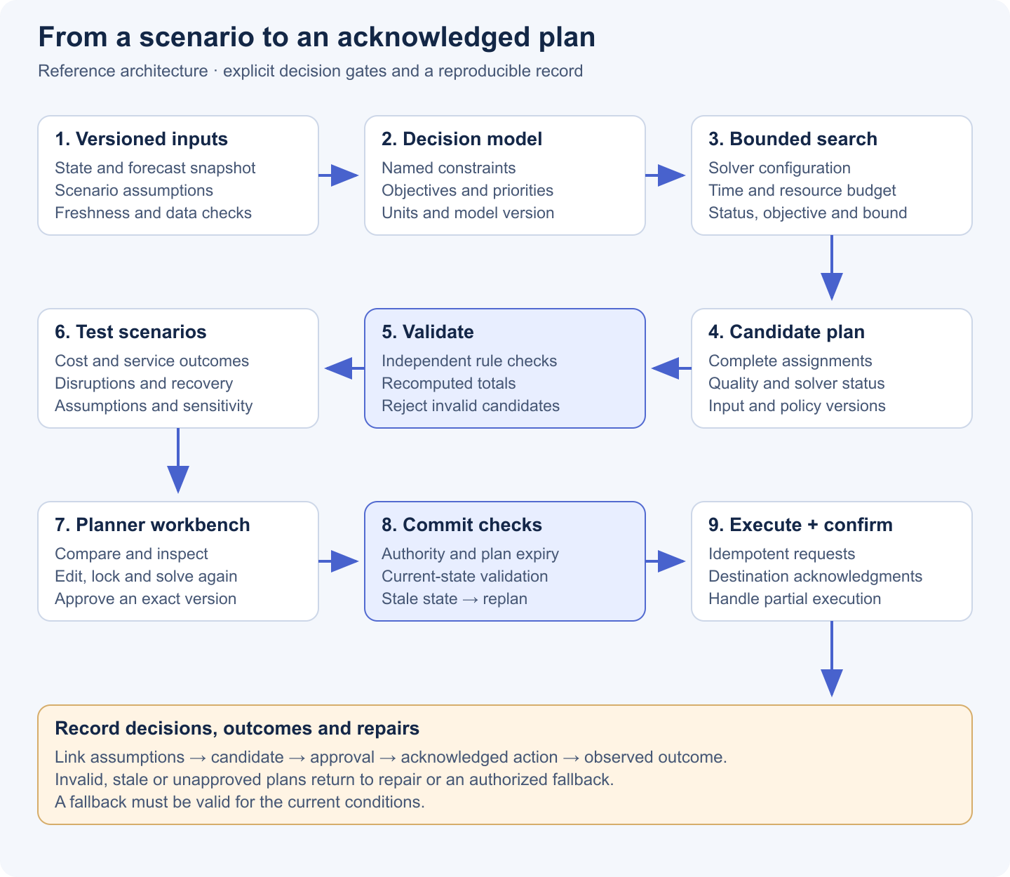
The planning service should produce a versioned candidate, together with its assumptions, objective components, solver status and constraint checks. A separate execution boundary decides whether that candidate may become an operational commitment.
Validate outside the solver’s output path
Independently check assignments, capacities, eligibility, totals and required commitments against the input snapshot. Recompute objective components where practical. This can catch serialization errors, rounding mistakes and integration defects that solver status alone cannot reveal.
The validator still depends on the completeness of its rules and the quality of its inputs. Reusing the same erroneous transformation in both components creates a shared blind spot. Test the validator with deliberately invalid plans and reconcile it with operational records.
Keep the model version, solver configuration, scenario version and candidate identity together. The user should be able to reopen a comparison and understand why a previous recommendation differs from today’s. Execution logs should identify the exact approved plan, not merely record that “optimization ran.”
6. Explain solver status without overstating certainty
“No plan returned” and “no feasible plan exists” are different findings. For example, OR-Tools CP-SAT distinguishes OPTIMAL, FEASIBLE, INFEASIBLE, MODEL_INVALID and UNKNOWN. FEASIBLE means a solution was found without proof of optimality; INFEASIBLE means infeasibility was proved. UNKNOWN can result when a limit is reached before those conclusions are established. Translate these states into distinct user actions. Source: OR-Tools solver documentation.
A timeout needs a conditional response
If a usable candidate exists, validate it and disclose that the search stopped before the desired proof or quality target. If no candidate exists, show the unresolved status and use the approved recovery path. Do not label a time-limited search “infeasible,” invent a plan, or execute incomplete assignments.
Where supported, expose the best feasible objective, the bound and the optimality gap. Gurobi’s relative MIP gap measures the difference between objective bounds relative to the incumbent objective; it is a solver quality criterion. It does not measure demand uncertainty or promise that realized cost will be within that percentage of the real-world optimum. Keep the model’s tolerances and termination conditions in the decision record. Source: Gurobi MIPGap reference.
Warm starts can help a new search reuse earlier work, but an earlier plan must still be checked against the new instance. Treat time budgets as part of the product contract, including time reserved for validation, review and execution.
7. Turn infeasibility into a repair workflow
Suppose committed orders require more capacity than the available fleet can supply within mandatory delivery windows. The product should identify the conflict, show the affected commitments and offer permitted changes. “Optimization failed” leaves the planner with the original problem and less time.
Diagnose first, relax only with authority
An irreducible inconsistent subsystem, or IIS, can isolate a conflicting subset of constraints and variable bounds. It is not necessarily the smallest such subset, and there may be several. It does not identify the cheapest or most acceptable business repair. If diagnosis is interrupted, its completeness also needs checking. Source: Gurobi model reference, computeIIS.
First check data defects and modeling mistakes. Then present authorized alternatives: acquire capacity, move a commitment with the customer’s agreement, or escalate a conflict to its owner. Show the impact of each alternative and rerun validation after the change.
A soft preference already modeled with a penalty can normally be violated without making the model infeasible. Lowering its penalty does not resolve contradictory hard constraints. If a diagnostic tool proposes relaxing a hard rule, treat that as a proposal requiring the appropriate authority, never as permission to cross the rule silently.
Save the chosen repair and its reason. Repeated conflicts may reveal a broken upstream promise, poor capacity data or a policy that needs business review.
8. Compare plans under uncertainty
A plan with the lowest nominal cost can become expensive when demand, travel time or equipment availability changes. Evaluate candidate plans under multiple conditions, using a consistent accounting horizon and explicit recovery assumptions.

In this example, plan B costs $800 more on an ordinary day but $4,800 less during disruption. With an assumed 20% disruption probability, its expected cost is $11,280, compared with $11,600 for A. The preference changes at a disruption probability of about 14.3%. That threshold gives the planner a concrete question: is the probability estimate credible enough to justify the extra reserve?
Test the assumptions behind the comparison
Two scenarios are useful for explanation, but rarely sufficient for deployment. Include correlated disruptions, extreme but plausible conditions, and failures of recovery resources. A spare vehicle is not useful if every depot is relying on the same spare. Evaluate service outcomes and constraint violations alongside monetary cost.
Stochastic optimization depends on its scenario distribution. Robust optimization protects against its specified uncertainty set. Neither provides protection against every event. Reserve scenarios not used to select the plan for evaluation, and distinguish empirical probabilities from deliberately adverse stress tests.
If using a simulator or digital twin, validate its behavior against observed operations in the intended operating range. Report where it is unreliable. Optimizing against an inaccurate simulator can produce a plan that exploits the simulator’s weaknesses instead of improving the business.
9. Give planners a decision workbench
The primary interface should make comparison easy: baseline beside alternatives, assumptions beside results, and operational changes beside the objective score. Include cost components, service levels, reserve capacity, unmet preferences, plan churn and solver status. Allow users to inspect the assignments behind each aggregate.
Make edits explainable and reversible
Let a planner lock an assignment, change an authorized assumption, or propose a constraint adjustment, then solve again. Show what changed and whether the edited plan remains feasible. A manual drag-and-drop action must not bypass validation simply because a human made it.
Explain bottlenecks carefully. A binding constraint is useful evidence, but does not by itself establish how much value removing it would create. Local sensitivity information can help for suitable continuous models; Gurobi documents dual values for convex continuous models and basis-dependent sensitivity ranges. For discrete choices, compare a newly solved scenario rather than presenting a continuous shadow price as a guaranteed marginal benefit. Source: Gurobi linear constraint attributes.
An LLM can translate “compare two fewer vehicles tomorrow” into a structured scenario proposal and explain verified results in plain language. Validate entity identifiers, units, ranges, permissions and business meaning, not just the JSON schema. Display the interpreted change for confirmation. The language model should draw numbers from the computed result and should not acquire execution authority through a conversational request.
10. Design execution and recovery together
Between calculation and approval, orders can change, stock can be reserved elsewhere and equipment can fail. Before committing, check plan expiry and the relevant state versions. If they differ materially, revalidate or replan. Use idempotent requests and record acknowledgments from the destination system so a retry cannot create duplicate commitments.
Replanning should respect work already underway
Freeze decisions that have become operational commitments, model the remaining work and limit unnecessary changes. Define which events trigger replanning and when a planner must intervene. An apparently cheaper plan can be worse once switching costs and disrupted execution are included.
Test recovery for solver outages, unavailable inputs, invalid outputs and partial execution. Yesterday’s plan is only a fallback if it remains valid now. Otherwise use a validated heuristic, a manual workflow or an approved hold procedure appropriate to the process. The agentic automation article covers authorization and durable execution in more detail.
Historical examples reinforce the need to distinguish recommendation quality from operational resilience. In December 2023, the US Department of Transportation announced a $140 million civil penalty for Southwest’s consumer-protection failures during and after its 2022 holiday disruption. DOT closed its separate unrealistic-scheduling investigation without a finding. This is not evidence that a particular optimizer caused the failure. Source: DOT’s 2023 announcement.
A December 2025 amended order credited the remaining $11 million Treasury installment for qualifying operational investments; it did not cancel the entire original penalty. The product lesson is to include recovery and customer communication in the operating design, while keeping the case’s legal findings and later developments accurate. Source: DOT’s 2025 order.
11. Evaluate the whole decision process
Replay historical decisions with only the information available at their planning time. Compare with the existing process under equal deadlines and constraints. Use the actual historical outcome to assess input forecasts, but recognize that an unexecuted alternative plan’s outcome usually requires a model or simulator. A favorable replay is not, by itself, causal proof of savings.
| Layer | Evidence to collect | What it establishes |
|---|---|---|
| Model and validation | Known-solution cases, deliberately invalid plans, unit checks, missing-rule reviews | The encoded decision behaves as intended on tested cases |
| Search performance | Feasible-plan rate, objective and bound, timeouts, latency by instance size | The service can deliver useful candidates within its budget |
| Scenario performance | Held-out conditions, service failures, recovery demand, sensitivity | The plan’s dependence on modeled assumptions |
| Human workflow | Review time, overrides and reasons, acceptance, edits and plan churn | Whether planners can understand and use the recommendation |
| Live operations | Acknowledged actions, realized cost, service outcomes, incidents | Whether execution produces value in the operating environment |
Swipe horizontally to read the complete table.
Move from shadow mode to a controlled pilot
Run recommendations without execution first, then pilot within a bounded operation. Where practical, use a comparison design that accounts for shared resources and spillovers; randomly assigning individual orders may be inappropriate when they share the same fleet. Predefine success, stop conditions and who can restore the established process.
Do not test operational safety by deliberately exceeding limits. Keep the independently engineered protection required by the process. Review overrides with planners: they may indicate missing constraints or local knowledge, rather than resistance to a better algorithm.
12. Measure value after execution
Build the business case from the decisions the product can influence. For a pre-launch estimate, model the gain per eligible decision, expected adoption, execution success and operating volume, then subtract software, compute, integration, review and maintenance costs. Show a range when these inputs are uncertain.
After launch, measure realized outcomes against a defensible comparison, adjusting for demand, prices and other material differences. If observed savings already reflect actual adoption, multiplying them by adoption again double-discounts the result. Check for displaced costs: one depot’s improvement may consume another depot’s capacity.
Use public cases as evidence of possibility
In March 2024, Walmart announced that its internally developed Route Optimization technology was available to other businesses. It reported eliminating 30 million unnecessary miles within its own operations. The announcement illustrates how an internal planning capability can become a product, but does not establish a transferable savings rate for another organization. Source: Walmart’s product announcement.
DeepMind’s 2016 account reported up to a 40% reduction in energy used for Google data-center cooling, not a 40% reduction in total data-center electricity. Its 2018 follow-up described direct control with local verification and operator override. These are useful precedents for combining learned response models with constrained decisions and a separate control boundary; they are not expected results for every planning product. Source: DeepMind’s 2016 report; 2018 control-system follow-up.
13. Release through evidence gates
Use capability gates rather than promising a universal implementation timeline. Complexity depends on the decision, data readiness, integration and consequences of a bad plan.
- Define the decision. Confirm the owner, objective, constraint inventory, baseline, deadline and execution boundary.
- Build the replayable model. Produce versioned snapshots, a simple baseline, candidate plans and independent validation. Resolve discrepancies with planners.
- Add comparison and repair. Support scenarios, honest solver states, infeasibility diagnosis, controlled edits and understandable tradeoffs.
- Prove operational readiness. Test stale inputs, outages, partial execution, recovery and plan changes in shadow mode and a bounded pilot.
- Expand on measured value. Broaden scope only after observed execution, service outcomes and economics justify it. Recheck assumptions as the operation changes.
A strong first release gives a planner a small set of credible options, enough evidence to choose among them, and a dependable way to carry out the chosen plan. More autonomy can follow when the operating evidence supports it.
The final article in this series turns to segmentation, personalization and recommendations: deciding which experience, offer or next step is useful for a particular user.
Sources and further reading
This article develops Chapter 11, “Scenario analysis and optimization,” of the AI Product Modernization Playbook supplied by Infinity Technologies. Architecture, product recommendations and the numerical comparison are editorial implementation guidance. The numerical example is hypothetical. Public case outcomes are attributed to their publishers and are not Infinity project results.
- Google OR-Tools: CP-SAT solver and result statuses.
- Gurobi: relative MIP optimality gap; IIS computation in the model reference; dual values and sensitivity attributes.
- Walmart: Route Optimization product announcement, March 2024.
- DeepMind: data-center cooling results, July 2016; autonomous control and verification, August 2018.
- US DOT: Southwest announcement, December 2023; amended order, December 2025.
Primary sources checked in October 2026. Product capabilities and operating conditions can change; validate the selected implementation against its current documentation and your own operating evidence.